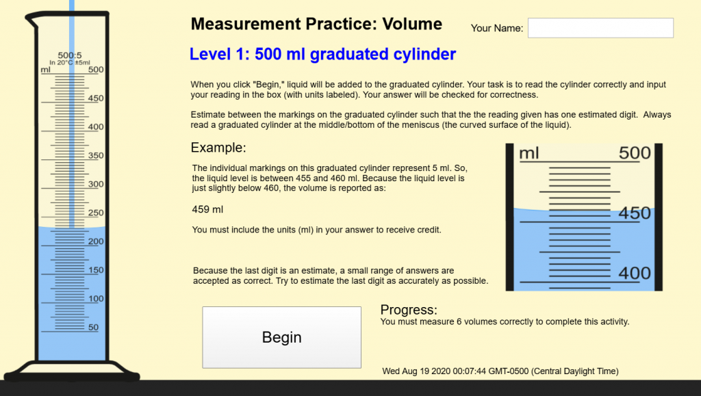
As we begin the school year in the wake of Covid-19, traditional labs and hands-on activities are very limited. Therefore, we need to find ways to do things virtually. I developed this interactive measurement & scale-reading activity using Construct 3. Students can use this to practice reading the scale on a ruler and reading the volume in three different-sized graduated cylinders.
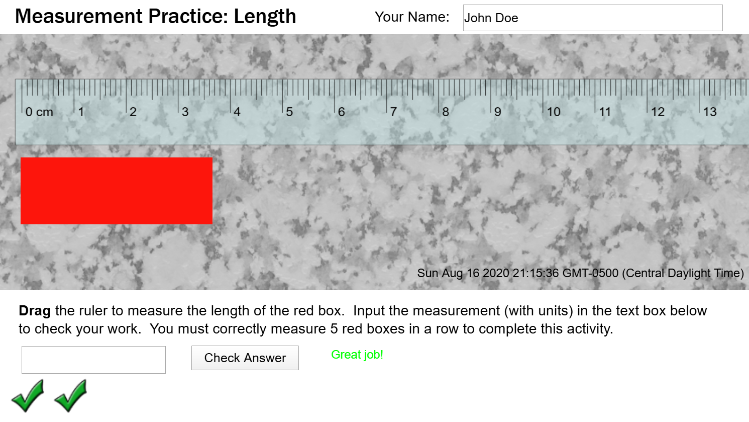
Length Measurement Features
Draggable ruler
Checks accuracy of measurement and provides feedback.
Accepts measurements within ±0.015 cm of the actual length.
Provides encouragement to estimate as accurately as possible for measurements within ±0.03 cm of the actual length.
Requires input of units (cm) for each measurement.
Challenges users to measure five lengths in a row. Any mistakes will cause the count to start over.
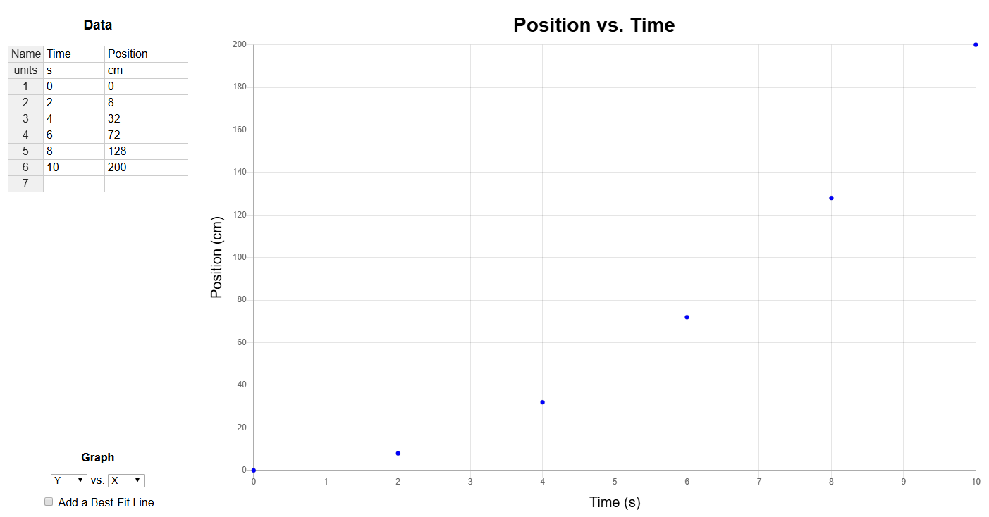
UPDATE: As of July 2020, I have updated the data analysis tool to use some cool newer JavaScript libraries. My graphing library is Chart.js (it has some fancy animation options and allows copy/pasting of generated graphs) and Handsontable (which uses an excel-like grid for inputting data, which also allows copy/pasting from excel or other spreadsheet programs).
Updated Data Analysis tool.
In Modeling Instruction and Advanced Placement science courses, students must be able to analyze data to determine the relationship between two variables. To make this easier, I created a Data Analysis Tool.
I’ve tried a few ways for students to graph data:
Method
Pros
Cons
Graph Paper
* Requires a firm grasp of scales, slope, and y-intercept * Students gain a better grasp of the meaning of these quantities and where they come from * Flexible — few limitations * No technology quirks to learn
* Time-consuming * Requires multiple iterations to linearize non-linear relationships * Difficult to test several analysis methods to determine the best fit * Best-fit lines, slopes, and y-intercepts are not as accurate
TI-84 Calculator
* Can be used on the AP Exam & ACT! * Manual window-setting requires students to consider how they will view their data * Students can create their own best-fit line by writing a linear equation in Y1 * OR, it has LinReg capabilities * A bit quicker than graphing by hand
* Data entry, turning stat-plots on, and graphing is not as intuitive as it could/should be * Regressions are also not very intuitive, and getting the linear fit to display on the graph is another hurdle * Doesn’t handle units at all — that’s up to the student * No easy way to get a printout of the graph for inclusion in reports * Not all students have this calculator (it’s expensive)
Vernier LoggerPro
* Quick * Takes care of units, labels, and titles * Easily adjust what is graphed on each axis * Support for force, motion, and other sensors * Linear fit is available with 1 button click * Supports graphing multiple data sets, a secondary y-axis scale, and many advanced features
* Linearizing with calculated columns is somewhat cumbersome; requires quite a few steps * For novices, the large number of features make it difficult to remember the correct steps to get the desired results * Not likely to use this software in other contexts * Not widely available (though the site license is generous)
Microsoft Excel or Google Sheets
* Powerful and flexible * Supports graphing multiple data sets, secondary y-axis scale, and many advanced features * Likely to be used in college, industry, etc. * Widely available (and for Google Sheets, free)
* Need to set up own data table * New versions of Excel do not label axes by default * Google Sheets graphs lack some features and are not the most intuitive (though I haven’t used them in a couple years so perhaps they’ve improved) * Again, the huge number of features often make it hard to find the desired functions
To start the year, I always have students graph data using graph paper for a couple weeks. I think students need to be able to do it themselves and understand the basic considerations of choosing scales, deciding what to plot where, and finding slopes and y-intercepts manually before having a device/computer do it for them.
In the past, after students got more comfortable graphing things by hand, I showed them how to use some tools (in the past, this tool has been LoggerPro). But, after having to guide students through the LoggerPro linearization process time and time again for each lab, I wanted to find a better solution. My current version works pretty well, but I’d welcome your feedback. I also have a version with linearization tools hidden.
Version 1.0
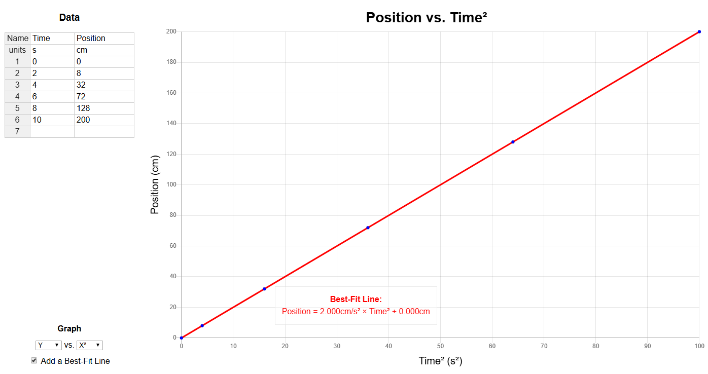
In June of 2016, I wrote a quick online data analysis tool (using the graphing capabilities of CanvasJS). Check it out here. It does most of what I need it to, which is to take a set of data, graph it, allow students to linearize it (graph y vs. x2, y vs. 1/x, etc.), and output the best-fit line equation.
Unit 1 of the Modeling Instruction chemistry curriculum has students develop the ideas of mass and volume and then the relationship between them (density). Consistent with the Modeling Instruction method, students collect data and analyze that data to develop a model to describe a relationship.
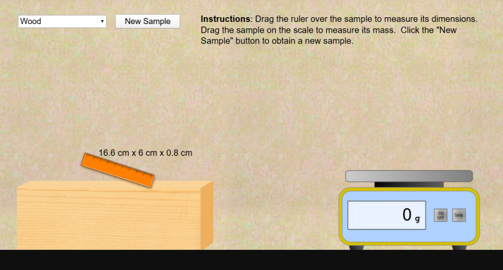
This year, my school is beginning virtually. It will be a challenge to transform our chemistry lab activities to the online format until we are able to resume in-person classes (and even then, we will be limited in the types of activities that we can do while “socially distant”). As I thought about facilitating my class online, I discovered Construct.net, which is typically used to produce online games. I found that it can be adapted to simulate labs like this one. I created a couple different versions. Check them out!
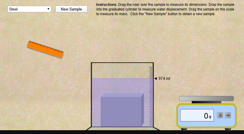
Dimensional Measurement VersionWater Displacement version
It simply allows students to measure the mass and volume of several samples of a material (currently, it has steel, aluminum, and wood). The first sample is always the same size for everybody, but subsequent samples are random sizes/masses (so encourage students to include a wide range of sample sizes in their data). Students can then use whatever graphing tools desired to analyze the data. A few years ago, I made a simple data analysis tool that would work well for this.
I like that the water displacement version shows which substances sink and float. Also, you can produce some samples that, because of their size or density (wood) do not completely submerge. This provides a chance to discuss what the water displacement measurement represents.
The water displacement version can also be used to show the relationship between cm3 and ml.
Just measure a sample with the ruler and then dunk it in the water.
Leave a comment about any issues you find or requests for features. Here are some things I’m thinking about:
More realistic interactions: an on-screen ruler to measure length, width, and height would build measurement skills. But, Contruct.net is really a 2-dimensional tool, so measuring that third dimension would be a challenge.
I had a request for cylindrical samples to better match the materials many of us use for the actual lab activity. It’s an idea for the future, especially if this is used to supplement the in-person activity for those who are absent.
UPDATE July 27, 2020:
Added zinc, copper, and lead to the substances.
Changed the button text to say “New Size”
Clarified the instructions.
The source files are available for anyone wanting to modify or extend. This was my first time using Construct.net, so keep that in mind before you berate me for my shoddy work 🙂. I do encourage anyone else working on this or similar lab simulations to share what you come up with.
LoggerPro functions for use in Calculated Columns. I always Google for this information and can never find it online. It is hidden in the “Help” for LoggerPro (who would think to look there!?).
Functions
– Trigonometric functions will use degrees or radians as set in the Settings for (file name) in the File menu.
(“X”, startRow, endRow) Takes all columns named “X” and extracts startRow to endRow for each of those columns, appending the values into a single column.
dataSets
datasets(“X”) Appends the dataset names of all datasets that have a column named “X”. Use analysis and datasets together to create a graph (analysis on the vertical axis and datasets on the horizontal). for example, if you had 3 datasets as follows: DS1 DS2 DS3 X X Y 1 11 21 2 12 22and then added analysis(“X”, 1, 1) and datasets(“X”) you would get:datasets analysis DS1 1 DS2 11
beats per minute
BeatsPerMinute(“Signal”, “Time”, intervalInSeconds, minPercent, maxPercent, noise) Returns the number of beats per minute of the values in “Signal” vs. “Time”. This function is similar to the rate function except that the interval given here is always in seconds and the returned value is always in minutes. For example, if “Time” is in seconds then: beatsPerMinute(“Signal”, “Time”, interval, min, max, noise) = 60 * rate(“Signal”, “Time”, interval, min, max, noise)
blood pressure
diastolic
The measured arterial pressure when the heart is at rest. “Pressure” and a “Time” column as inputs and return a single number. diastolic(“Pressure”, “Time”) “Pressure”: Pressure values from the BPS “Time”: Time the pressure values were recorded Returns the smaller number of blood pressure
meanArterialPressure
meanArterialPressure(“Pressure”, “Time”)“Pressure”: Pressure values from the BPS “Time”: Time the pressure values were recorded Returns the pressure value at the max peak used for blood pressure calculations.
Oscillations
Oscillations(“Pressure”, “Time”) “Pressure”: Pressure values from the BPS “Time”: Time the pressure values were recorded Returns the Oscillations of the peaks and valleys used to calculate systolic and other blood pressure values.
OscillatoryPeaks
OscillatoryPeaks(“Pressure”, “Time”) “Pressure”: Pressure values from the BPS “Time”: Time the pressure values were recorded Returns the peaks used to calculate systolic, diastolic, and pulse (the “high” values in “Oscillations”).
pulse
pulse(“Pressure”, “Time”) “Pressure”: Pressure values from the BPS “Time”: Time the pressure values were recorded Returns the pulse using the inputs from the Blood Pressure Sensor (similar results, different algorithm as the other beats-per-minute functions)
systolic
systolic(“Pressure”, “Time”) “Pressure”: Pressure values from the BPS “Time”: Time the pressure values were recorded The measured arterial pressure when the heart contracts. Returns the larger number of blood pressure
boolean
For the boolean functions a 1 is considered true, 0 false and anything else an invalid input
AND
AND(X, Y) return 1 if and only if X and Y are both 1
NOT
NOT(X) return 1 if X is 0; 0 if X is 1
OR
OR(X, Y) return 1 if X or Y is 1
XOR
XOR(X, Y) return 1 if X or Y is 1 but not both
calculus
calculus >
derivative
derivative(“Y”, “X”) “Y”: A column of real numbers “X”: Optional. A column of real numbers The numerical derivative is the weighted average of the slope of ‘n’ points around each point. You can set ‘n’ in Settings for (Name). If you don’t supply an “X” column, the program will find one.
derivativeSG
derivativeSG(“Y”, “X”) “Y”: A column of real numbers “X”: Optional. A column of real numbers Savitsky-Golay derivative. Fits a polynomial to ‘n’ points around each point and computes the derivative of the polynomial at that point. You can set ‘n’ in Settings for (Name). If you don’t supply an “X” column, the program will find one.
derivativeTimeShift
derivativeTimeShift(“Y”, “X”) Returns the derivative of “Y” with respect to “X”. This function is specifically designed to be used with photogate and picket fence data. The derivatives returned are adjusted to estimate values at the start of the timing interval, instead of the midpoint. For details see The Physics Teacher, Vol 35, April 1997, p. 220. The article written by William Leonard is entitled “The Dangers of Automated Data Analysis.” Average velocity during the time interval is equal to the instantaneous velocity at midpoint of the time interval. Where
integral
integral(“Y”,”X”) “Y”: A column of real numbers “X”: Optional. A column of real numbers The numerical integral is the running sum of the areas of rectangles calculated by the midpoint rule. The i’th rectangle is (Yi – Y(i-1)) / (Xi – X(i-1)). If you don’t supply an “X” column, the program will find one.
secondderivative
secondDerivative(“Y”, “X”) “Y”: A column of real numbers “X”: Optional. A column of real numbers Calculates the numerical second derivative of “Y” with respect to “X”. If you don’t supply an “X” column, the program will find one.
secondderivativeSG
secondDerivativeSG(“Y”, “X”) “Y”: A column of real numbers “X”: Optional. A column of real numbers Savitsky-Golay second derivative. Fits a polynomial to ‘n’ points around each point and computes the second derivative of the polynomial at that point. You can set ‘n’ in Settings for (Name). If you don’t supply an “X” column, the program will find one.
secondderivative Time Shift
secondDerivativeTimeShift(“Y”, “X”) “Y”: A column of real numbers “X”: Optional. A column of real numbers Numerical time-shifted second derivative. Calculates the second numerical derivative of “Y” with respect to “X”. The values are shifted so that the derivatives are calculated at the midpoints between each two values. If you don’t supply an “X” column, the program will find one.
collapse
collapse(“X”) Returns a column with all non-numerical cells (blanks and text) removed.
collapseIndirect
collapseIndirect(X, Y) Returns a column of only the rows in “X” corresponding to rows in “Y” that have valid numerical cells.
constant
Constant(x, num) x: A real number num: A real number or a column Generates a constant column filled with the value ‘x’. The number of values in the returned column is num, or if a column was passed in, the size of the passed-in column.
delta
delta (“X”) “X”: A column of real numbers Returns a column of values where the i’th value is the i’th value in “X” minus the (i-1)’th value in “X”.
digital filtering
lowPassFilter
(“Y”, “X”, “ripple”, “freqCutoff”) “Y”: The data column to be filtered “X”: The associated time column for “Y” “ripple”: The ripple allowed in the pass-band “freqCutoff”: Cut-off frequency (-3dB), in hertz Applies a Chebyshev low-pass filter. For “ripple”, enter a value that is a percent of the pass-band. To apply a Butterworth low-pass filter, set “ripple” to 0.
highPassFilter
(“Y”, “X”, “ripple”, “freqCutoff”) “Y”: The data column to be filtered “X”: The associated time column for “Y” “ripple”: The ripple allowed in the pass-band “freqCutoff”: Cut-off frequency (-3dB), in hertz Applies a Chebyshev high-pass filter. For “ripple”, enter a value that is a percent of the pass-band. To apply a Butterworth high-pass filter, set ripple to 0.
bandPassFliter
(“Y”, “X”, “lowFreq”, “highFreq”) “Y”: The data column to be filtered “X”: The associated time column for “Y” “lowFreq”: Low frequency cut-off (-3dB), in hertz “highFreq”: High frequency cut-off (-3dB), in hertz Ripple is automatically set to zero and is not adjustable. The function returns the signal with the frequencies outside the designated frequency range removed.
bandStopFliter
(“Y”, “X”, “lowFreq”, “highFreq”) “Y”: The data column to be filtered “X”: The associated time column for “Y” “lowFreq”: Low frequency cut-off (-3dB), in hertz “highFreq”: High frequency cut-off (-3dB), in hertz Ripple is automatically set to zero and is not adjustable. The function returns the signal with the frequencies inside the designated frequency range removed.
timeDecayFilter
(“Y”, “X”, “decayConstant”) “Y”: The data column to be filtered “X”: The associated time column for “Y” “decayConstant”: A value in seconds that determines the decay of “Y” Applies an exponential time decay to the signal.
ElectrophoresisInterpolate
ElectrophoresisInterpolate(“Std. Dist”, “Std. BP”, “Dist”) “Std. Dist”: Distances from the standard “Std. BP”: Base Pair Counts from the standard “Dist”: Distances to interpolate Returns a column of base pair counts based on the Electrophoresis curve fit for “Std. Dist” vs. “Std. BP” given “Dist”. Will NOT work if curve fit has been deleted. This function is used automatically when doing a Gel Analysis (Electrophoresis).
exp
exp(“X”) “X”: A column of real numbers Returns the exponent, exp(x) = e^x, where e is the natural log base (2.17…).
integer
integer(“X”) Extracts the integral part of values in “X”.
interpolate
interpolate(“X”) Fills in missing values using linear interpolation.
ln
ln(“X”) “X”: A column of real numbers larger than 0 Returns the natural logarithm. If b = ln(a) then e^b = a (Where e is the constant 2.17…).
log
log(“X”) “X”: A column of real numbers larger than 0 (Log base 10) If b = log(a) then 10^b = a.
modulo
modulo(“X”, n) “X”: A column of integers n: An integer larger than 0 Returns the remainder of each of the numbers in “X” when divided by n.
photogate
Blocked MidTimes
BlockedMidTimes(“Time”, “Gate1”, “Gate2”) “Time”: Optional. A column of real numbers (the times of events) “Gate1”: A column of photogate states (1’s and 0’s) “Gate2”: Optional. A column of photogate states (1’s and 0’s) Calculate the average times between blocked events from Gate 1 to Gate 2. If you don’t enter a “Time” column, the program will find one. If you don’t enter “Gate2”, “Gate1” will be used.
Blocked to Blocked
BlockedToBlocked(“Time”, “Gate1”, “Gate2”) “Time”: Optional. A column of real numbers (the times of events) “Gate1”: A column of photogate states (1’s and 0’s) “Gate2”: Optional. A column of photogate states (1’s and 0’s) Returns a column of the times between successive blocked events in gate 1 and blocked events in gate 2. If you don’t enter a “Time” column, the program will find one. If you don’t enter “Gate2”, “Gate1” will be used.
Blocked to Unblocked
BlockedToUnblocked(“Time”, “Gate1”, “Gate2”) “Time”: Optional. A column of real numbers (the times of events) “Gate1”: A column of photogate states (1’s and 0’s) “Gate2”: Optional. A column of photogate states (1’s and 0’s) Returns a column of the times between successive blocked events in gate 1 and unblocked events in gate 2. If you don’t enter a “Time” column, the program will find one. If you don’t enter “Gate2”, “Gate1” will be used.
Blocked to Unblocked MidTimes
Blocked to Unblocked MidTimes “Time”: Optional. A column of real numbers (the times of events) “Gate1”: A column of photogate states (1’s and 0’s) “Gate2”: Optional. A column of photogate states (1’s and 0’s) Calculate the average time between the blocked events in gate 1 and unblocked events in gate 2. If you don’t enter a “Time” column, the program will find one. If you don’t enter “Gate2”, “Gate1” will be used.
derivativeTimeShift
DerivativeTimeShift (“Y”, “X”) Returns the derivative of “Y” with respect to “X”. This function is specifically designed to be used with photogate and picket fence data. The derivatives returned are adjusted to estimate values at the start of the timing interval, instead of the midpoint. For details see The Physics Teacher, Vol 35, April 1997, p. 220. Average velocity during the time interval is equal to the instantaneous velocity at midpoint of the time interval. Where
Pendulum Period
PendulumPeriod(“Time”, “Gate1”) “Time”: Optional. A column of real numbers (the times of events) “Gate1”: A column of photogate states (1’s and 0’s) Calculate the time between every other blocked event on Gate 1. If you don’t enter a “Time” column, the program will find one.
secondDerivativeTimeShift
secondDerivativeTimeShift(“Y”, “X”) “Y”: A column of real numbers “X”: Optional. A column of real numbers Numerical time-shifted second derivative. Calculates the second numerical derivative of “Y” with respect to “X”. The values are shifted so that the derivatives are calculated at the midpoints between each two values. If you don’t supply an “X” column, the program will find one.
Unblocked to Blocked
UnblockedToBlocked(“Time”, “Gate1”, “Gate2”) “Time”: Optional. A column of real numbers (the times of events) “Gate1”: A column of photogate states (1’s and 0’s) “Gate2”: Optional. A column of photogate states (1’s and 0’s) Returns a column of the times between successive unblocked events in gate 1 and blocked events in gate 2. If you don’t enter a “Time” column, the program will find one. If you don’t enter “Gate2”, “Gate1” will be used.
Unblocked to Unblocked
UnblockedToUnblocked(“Time”, “Gate1”, “Gate2”) “Time”: Optional. A column of real numbers (the times of events) “Gate1”: A column of photogate states (1’s and 0’s) “Gate2”: Optional. A column of photogate states (1’s and 0’s) Returns a column of the times between successive unblocked events in gate 1 and unblocked events in gate 2. If you don’t enter a “Time” column, the program will find one. If you don’t enter “Gate2”, “Gate1” will be used.
Unblocked to Blocked MidTimes
Unblocked to Blocked MidTimes “Time”: Optional. A column of real numbers (the times of events) “Gate1”: A column of photogate states (1’s and 0’s) “Gate2”: Optional. A column of photogate states (1’s and 0’s) Calculate the average time between unblocked events in gate 1 and blocked events in gate 2. If you don’t enter a “Time” column, the program will find one. If you don’t enter “Gate2”, “Gate1” will be used.
Unblocked MidTimes
UnblockedMidTimes(“Time”, “Gate1”, “Gate2”) “Time”: Optional. A column of real numbers (the times of events) “Gate1”: A column of photogate states (1’s and 0’s) “Gate2”: Optional. A column of photogate states (1’s and 0’s) Calculate the average times between unblocked events from Gate 1 to Gate 2. If you don’t enter a “Time” column, the program will find one. If you don’t enter “Gate2”, “Gate1” will be used.
rate
rate(“Y”, “X”, t, m1, m2, n) “Y”: A column of real numbers “X”: Optional. A column of real numbers t: Optional. Time interval m1: Optional. Minimum threshold m2: Optional. Maximum threshold n: Optional. Noise threshold Returns the rate of “Y” with respect to “X”, where t is the time interval measured, m1 is min percentage threshold, m2 is max percentage threshold, and n is noise threshold. “X”, t, m1, m2, and noise are all optional with default values “X” is time column, t = 1/10 the range, m1 = 40%, m2 = 60%, and noise = 0. Details
rotary motion
amplitude
(“Data Column”, “Time Column”, “Min Percent”, “Max Percent”, “Time Interval”) “Data Column”: Data for which you want to calculate amplitude “Time Column”: Associated time column for “Data Column” “Min Percent”: Threshold used to detect valleys “Max Percent”: Threshold used to detect peaks “Time Interval”: Period of time over which amplitude is calculated (in the time units of the experiment) Calculates peak to peak amplitude. For Min and Max Percent, enter values between 0 and 100. Smaller values are more sensitive to noise and thus more sensitive to real cycles. Larger values are less sensitive to noise; too large of a value may filter out real cycles. “Time Interval” ends at the row at which the value is calculated (the current time).
period
(“Data Column”, “Time Column”, “Min Percent”, “Max Percent”, “Time Interval”) “Data Column”: Data for which you want to calculate period “Time Column”: Associated time column for “Data Column” “Min Percent”: Threshold used to detect valleys “Max Percent”: Threshold used to detect peaks “Time Interval”: Period of time over which period is calculated (in the time units of the experiment) Calculates the period of an oscillating function. For Min and Max Percent, enter values between 0 and 100. Smaller values are more sensitive to noise and thus more sensitive to real cycles. Larger values are less sensitive to noise; too large of a value may filter out real cycles. “Time Interval” ends at the row at which the value is calculated (the current time).
round
round(“X”) “X”: A column of real numbers Round. Returns the closest integer to x. If x is equidistant to two integers, round(x) gives the largest of the two (e.g., round(0.5) = 1).
smoothAve
smoothAve(“X”) “X”: A column of real numbers Returns a column of moving averages of the values in “X”. The width of the “window” to use when averaging points can be set in Settings for (Name)…
statistics
abs
abs(“X”) “X”: A column of real numbers Absolute value. If x less than 0, then abs(x) = -x. Otherwise, abs(x) = x.
ceiling
ceiling(“X”) “X”: A column of real numbers Returns the smallest integer larger than or equal to x.
floor
floor(“X”) “X”: A column of real numbers Returns the largest integer smaller than or equal to x.
max
max(“X”) “X”: A column of real numbers Compares all the values in a single column and returns a single number-the largest number in the column.
max2
max2(“X”, “Y”) “X”: column of real numbers “Y”: A column of real numbers or a single number. Compares all the values in a column against a real number (e.g max2(“X”, 5.1))
mean
mean(“X”) “X”: A column of real numbers Arithmetic mean. Returns the sum of all the values in “X” divided by the number of values.
median
Median(“X”). “X”: A column of real numbers If m = median(“X”), then half the numbers in “X” are greater than (or equal) to m, and half are less than or equal.
min
min(“X”) “X”: A column of real numbers Compares all the values in a single column ,and returns a single number-the smallest number in the column.
min2
min(“X”, “Y”) “X”: A column of real numbers “Y”: A column of real numbers or a single number Compares all the values in a column against a real number (e.g min2(“X”, 5.1))
numRows
NumRows(“X”) “X”: A column of real numbers Returns a single value-the number of rows in the column.
randInt
randInt(min, max, num): min: A real number max: A real number num: A real number or a column Random Integer. Returns a column of random integers between min and max (inclusive). The size of the returned column is num. If num is a column, then the size will be the number of rows in that column.
randReal
randReal(min, max, num) min: A real number max: A real number num: A real number or a column Random Real. Returns a column of random real numbers between min and max (inclusive). The size of the returned column is num. If num is a column, then the size will be the number of rows in that column.
stddev
stddev(“X”) “X”: A column of real numbers Standard Deviation. Returns a column representing the standard deviations of each of the numbers in a column.
step
step(start, increment, num, first, skip) start: Start value increment: Increment value num: Number of values to generate first: Optional. First non-empty row skip: Optional. Rows to skip between each value Generates a column “num” rows long starting with “start” and incrementing by “increment”. “num” can be a positive integer or a column name. Optional parameters: “first” is the first non-empty row and “skip” is the number of rows to skip between each value.
StepColumnBase
stepColumnBased(“X”, start, increment, first, skip) start: Start value increment: increment value first: Optional. First non-empty row skip: Optional. Row to skip between each value Generates a column based on non-empty values in column “X” starting with “start” and incrementing by “increment.” “First” is the first non-empty row and “skip” is the number of rows to skip between each value.
subset
subset(“X”, startRow, step) “X”: A column of real numbers startRow: An integer larger than 0 step: An integer larger than 0 Extract a subset. Returns a column extracted from “X” starting with ‘startRow’ by ‘step’. For example, subset(“X”, 1, 2) will get every second row of “X” starting with row 1.
sum
Sum(“X”) “X”: A column of real numbers Returns a column whose n’th value is the sum of the values in “X” from row 1 to n.
sqrt
Square root. “X”: A column of non-negative real numbers. If x is the square root of y, then x*x = y.
trigonometric
sin
sin(“X”) “X”: A column of real numbers In a right triangle with angle between two sides ‘x’, sin(x) is the length of the opposite side divided by the hypotenuse.
cos
cos(“X”) “X”: A column of real numbers In a right triangle with angle between two sides ‘x’, cos(x) is the length of the adjacent side divided by the hypotenuse.
tan
tan(“X”) “X”: A column of real numbers In a right triangle with angle between two sides ‘x’, tan(x) is the length of the opposite side divided by the adjacent side.
asin
asin(“X”) “X”: A column of real numbers between -1 and 1 Arcsine function. asin(x) = the angle whose sine is x.
acos
acos(“X”) “X”: A column of real numbers between -1 and 1 Arccosine function. acos(x) = the angle whose cosine is x.
atan
atan(“X”) “X”: A column of real numbers Arctangent function. atan(x) = the angle whose tangent is x. The result will be between -pi/2 and pi/2.
sinh
sinh(“X”) “X”: A column of real numbers Hyperbolic sine.
cosh
cosh(“X”) “X”: A column of real numbers Hyperbolic cosine.
tanh
tanh(“X”) “X”: A column of real numbers Hyperbolic tangent.
Value
Value(n, “X”) n: Number of rows backwards (when n < 0) or forwards (n >0) in column “X” to extract a value from. “X”: Column from which to extract values . Create a new column from another column by extracting offset values.
If data are imported from an experiment file, you may want to specify the independent column. For example, if the imported data included “time” in the first column but you wanted to calculate the derivative of pH with respect to volume, you have to define the derivative as derivative(“pH”,”Volume”).
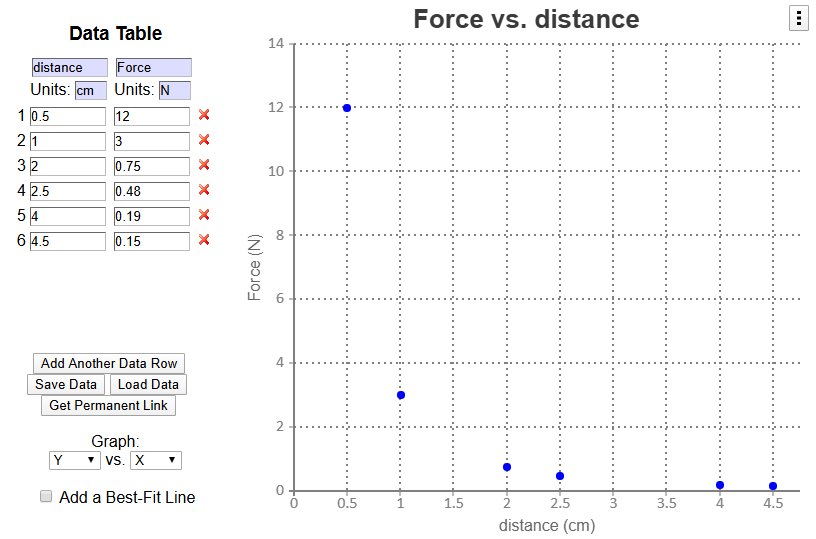
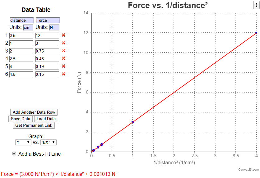
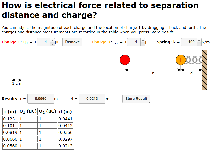
In the Modeling Instruction materials for Physics: E&M, there are videos provided that can be analyzed to develop quantitative relationships between electrostatic force, separation distance, and charge quantity. However, this process is rather complex and requires using distance as a proxy for force. While the inverse-square relationship comes out (though even that can be difficult to determine if students aren’t very careful about the video analysis), it does not allow for a determination of the Coulomb constant, since the charge of the objects in the video is not known.
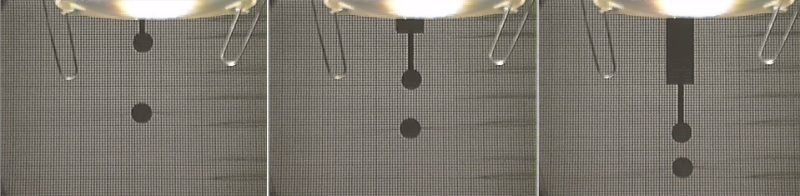
Using actual charged pith balls and measuring repulsion.
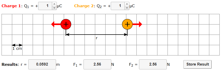
To try to remove some of the difficulties while still using the data analysis to develop model for electrostatic force interactions, I developed a simulation that allows a more direct “measurement” of charge, distance, and force.
As part of my action research project for my Master of Natural Science degree from Arizona State University (home of Modeling Instruction), my research partner Mr. Wirth and I looked at how we could apply computational modeling at several key points in the curriculum to improve students’ understanding of physics.
We worked with a small sample group, but we had some promising results. Spreadsheets allowed students to solve more complex problems than can typically be solved in a first-year physics course. Spreadsheets freed students a bit to think about the problem rather than focusing on the computation, though learning to graph and write equations in excel was challenging.